Tutorial on benchmarking machine learning potentials
This tutorial shows how to evaluate various machine learning potentials (MLPs) within the MLatom framework. You can use this tutorial to either benchmark MLatom-supported MLPs for your own application or you can interface any other 3rd party MLP to MLatom to compare this MLP’s performance to those we benchmarked in:
Max Pinheiro Jr, Fuchun Ge, Nicolas Ferré, Pavlo O. Dral, Mario Barbatti. Choosing the right molecular machine learning potential. Chem. Sci., 2021, 12, 14396–14413. DOI: 10.1039/D1SC03564A. (blog post)
Machine learning potentials (MLPs) provide us a pathway to greatly reduced the number of quantum chemical calculations for some data-hungry applications like molecular dynamics, geometry optimization, absorption, and emission spectra simulation, etc. Nevertheless, we might get lost in the wide selection of MLP models, from which picking up the right one is error-prone. Yet to mention the tedious affairs such as the format conversion for your data input. Here is just a selection of some popular types of MLPs (see above paper for a wider overview):

To make the life easier, we provide the MLatom 2, An Integrative Platform for Atomistic Machine Learning, which automates the performance evaluation for some typical MLP models on an equal footing. One of the key elements in a fair comparison of MLPs is evaluating how their generalization error (error in the test set) depend on the increased number of the training points, i.e., comparing their learning curves rather than making a comparison on the same number of training points (the curves may cross and that’s why comparison on a single point will not give you a full picture). Another point is to count the validation set used for choosing hyperparameters or early stopping as part of the training set, because the validation set is indirectly used for training. Finally, if the training and prediction time is of interest, calculations should be performed on the same hardware architecture with the same number of CPUs/GPUs, as comparing timings reported on very different architectures is like comparing apples with oranges.
Specifically, we archived this goal by introducing the interfaces and the task learningCurve.
The idea of interfaces is to use agents that communicate between MLatom and 3rd-party programs, with translated data back and forth. Therefore, the MLatom’s data format can be seamlessly used to train other MLPs, and the analysis function in MLatom can give detailed reports on their performance.
So far, we’ve interfaced 5 popular implementations of different MLP models. These models are:
- ANI (through TorchANI)
- DeepPot-SE and DPMD (through DeePMD-kit)
- GAP–SOAP (through GAP suite and QUIP)
- PhysNet (through PhysNet)
- sGDML (through sGDML)
They covered all the categories shown in the figure above.
To get such a curve, we have to repeatedly test the trained models, ideally, also many times for the same number of training points to get the standard deviation (“error bar”) of the test error. Now the whole process is packed into a single task: learningCurve, which will do all the training and summarize the results for you.
Want to have a try? This tutorial is going to tell you how to use these features.
Now, let’s get to it!
Table of Contents
Preparations before you start
To follow this tutorial, you need:
The latest version of MLatom (version 2.0.3 is recommended if you want to run with the same settings as in our manuscript above), which you can get from here.
Third-party MLP programs that you want to test. The installation guide can be found here. After the 3rd-party programs are installed and accessible through environment variables, we can use MLatom to invoke them.
Necessary dataset files. Here we’ll use the MD17 dataset, which can be downloaded from quantum-machine.org. This data set is inthe Extended XYZ (extXYZ) format. Here are the links for molecules in the dataset:
Zipped files for this tutorial and reproducing our benchmark results. You can download it from figshare (384.76 MB!).
After the MD17_lite.7z is unzipped, you’ll get 10 folders for 10 organic molecules in MD17 dataset. And you need to extract extXYZ dataset files of each molecule to the corresponding folder.
Inside each folder, execute:
../converting-to-MLatom-format.py
To convert the extXYZ file to separate xyz.dat, en.dat, and grad.dat.
Then:
../get_lite_dataset.py
To get the lite version of datasets (with 20k test points) that we actually used in our project based on the idx_lite.dat.
Make sure above Python 3 scripts have right permissions to be executed.
Using MLPs
Generally, we have two ways to train and use MLPs in MLatom. One way is specifying the MLP model with the keyword MLmodelType in the program input. The other way is using the keyword MLprog to specify which program to use. The default ones are native implementations in MLatom (KREG in MLatomF).
The available values for MLmodelType and MLprog are shown in the table below:
Supported ML model types and default programs:

Supported interfaces with default and tested ML model types:

You can use MLatom.py MLmodelType help or MLatom.py Mprog help to print out the ASCII table above.
Basically, you just need to change a couple of lines to choose an MLP model of your interest. Here is an example input for calculating the test error:
estAccMLmodel			# task to estimate the accuracy of a ML model
XYZfile=../xyz.dat_lite		# data file stores molecular geometries in XYZ format.
Yfile=../en.dat_lite		# data file stores molecular energies
Ntrain=100			# number of geometries to be used for training
Ntest=20000			# number of geometries to be used for testing
MLmodelType=[your model] 	# in principle, this is the only line you need to change!
Some models may require some other model-specific options to be specified. Below we briefly overview the models and point out some important model-specific options.
Kernel method (KM) based MLPs
KREG
The KREG model is one of the natively implemented models in MLatom.
The name KREG came from the combo of kernel ridge regression (KRR) algorithm, RE descriptor, and Gaussian kernel.
The RE descriptor consists of inversed distances between every two atoms in the molecule, but normalized to the equilibrium geometry. Since the RE descriptor describes the molecule as a whole, it belongs to the global descriptors.
More details about the KREG model can be found in MLatom 2 paper.
By default, the KREG model will be used if MLmodelType and MLprog is no specified.
Here’s an example input for using the KREG mode (ethanol/KREG/KREG.inp in the zip file):
estAccMLmodel
XYZfile=../xyz.dat_lite
Yfile=../en.dat_lite
Ntrain=1000
Ntest=1000
sigma=opt
lambda=opt
The last two lines specified the two hyperparameters in the KREG model to be optimized to get the more accurate model.
You can check the manual and other tutorials to know more about the KREG model!
GAP
The Gaussian approximation potential (GAP) is a kernel method-based MLP model that uses Gaussian process regression (GPR) as its fundamental algorithm. It is usually combined with a local type descriptor call SOAP (smooth overlap of atomic positions). We interfaced them through QUIP and GAP suite programs.
To access this model in MLatom, just add MLmodelType=GAP-SOAP or MLprog=GAP in the input.
Here’s a sample input file (ethanol/gap/gap.inp):
estAccMLmodel
XYZfile=../xyz.dat_lite
Yfile=../en.dat_lite
Ntrain=100
Ntest=900
MLmodelType=GAP-SOAP 		# or MLprog=GAP
You can go to the directory where the input file is unzipped and run it with:
MLatom.py gap.inp
If everything goes well, you’ll get a screen output similar to gap.out.
Of course, you can access the options that the original programs provide.
For example, in the input script, you can use gapfit.gap.cutoff to set the cutoff radius for local atomic environments.
You can check more options with MLatom.py MLProg=GAP help.
GDML and sGDML
The gradient-domain ML (GDML) and its symmetrized version (sGDML) is another KM based model we interfaced. Both of them use KRR with a global descriptor that comes from unnormalized inverse distances for every two atoms (ID descriptor, which is similar to the RE descriptor). As their names suggest, the information of gradients (e.g. forces, which are the negative gradients of energies) is required.
We interfaced GDML and sGDML through the sGDML program. And here’s a sample input (ethanol/sgdml/sgdml.inp):
estAccMLmodel
XYZfile=../xyz.dat_lite
Yfile=../en.dat_lite
YgradXYZfile=../grad.dat_lite
Ntrain=100
Nsubtrain=80
Nvalidate=20
Ntest=900
MLmodelType=sGDML
Notice that here we also specify Nsubtrain and Nvalidate, because the sGDML program has built-in optimization for hyperparameters. If you don’t specify these numbers, the default ones will be used.
To use GDML model, you need to set sgdml.gdml=True or MLmodelType=GDML.
Check more options with MLatom.py MLProg=sGDML help.
Neural Network (NN) based MLPs
ANI
The next model to introduce is ANI, whose name is the second-order abbreviative of Accurate NeurAl networK engINe for Molecular Energies. (Hint: the first-order one is ANAKIN-ME.)
Anyway, different from the two MLPs above, ANI is a neural network-based model. ANI model consists of a fixed local descriptor call atomic environmental vector (AEV), which is derived from the descriptor in Behler and Parrinello’s work. We interfaced the package TorchANI to make the ANI model available in MLatom.
Sample input (ethanol/ani/ani.inp):
estAccMLmodel
XYZfile=../xyz.dat_lite
Yfile=../en.dat_lite
Ntrain=100
Nsubtrain=80
Nvalidate=20
Ntest=900
MLmodelType=ANI
ani.max_epochs=100
We can train an ANI model in MLatom with the input above.
Since ANI is a NN based model, there are lots of NN-related hyperparameters that can be tuned. E.g., the last line in the input specifies the halting condition for NN training with 100 epochs at maximum. Otherwise, it will keep running until the default conditions are met, which is too far for this tutorial.
Check more options with MLatom.py MLProg=TorchANI help.
DeepPot-SE and DPMD
Deep Potential – Smooth Edition (DeepPot-SE) and its predecessor Deep Potential Molecular Dynamics (DPMD) are interfaced through their official implementation: DeePMD-kit. These two models are NN based too, but DeepPot-SE includes a learned local descriptor rather than the fixed one in DPMD.
Sample input (ethanol/deepmd/deeppot-se.inp):
estAccMLmodel
XYZfile=../xyz.dat_lite
Yfile=../en.dat_lite
Ntrain=100
Nsubtrain=80
Nvalidate=20
Ntest=900
MLmodelType=DeepPot-SE
deepmd.training.stop_batch=2000
To use DPMD model, you need to set MLmodelType=DPMD.
Check more options with MLatom.py MLProg=DeePMD-kit help.
PhysNet
PhysNet is another NN based model we interfaced. It also uses a learned local descriptor as DeepPot-SE does.
Note that the original implementation of PhysNet is programmed in Python 3.6 with TensorFlow v1, to make it compatible with the newer platform. We need to do some minor modifications that are described in the installation guide.
Sample input (ethanol/physnet/ physnet.inp):
estAccMLmodel
XYZfile=../xyz.dat_lite
Yfile=../en.dat_lite
Ntrain=100
Nsubtrain=80
Nvalidate=20
Ntest=900
MLmodelType=PhysNet
physnet.max_steps=100
Check more options with MLatom.py MLProg=PhysNet help.
Detailed lists of tunable hyperparameters for each 3rd-party program can also be found in the paper of MLatom 2.
Optimizing hyperparameters through hyperopt interface
The optimization for hyperparameters is a critical problem for ML. Tuning them manually is not an ideal and reliable way.
Hence, (especially after 3rd-party programs being introduced,) we also interfaced a program call hyperopt to automatically search the hyperparameters’ spaces and give the best possible values.
To enable the optimization with hyperopt, we just need to substitute the value of the keyword to a function-like string hyperopt.xxx(), where xxx defines the shape of the searching space. Available shapes are:
hyperopt.uniform(lb,ub): linear search space from lower bound lb, and upper bound ub.hyperopt.loguniform(lb,ub): logarithmic search space, base 2.hyperopt.qunifrom(lb,ub,q): discrete linear space, rounded by q
Once the function-like string is present in the input script, the hyperopt will be enabled. And the option hyperopt.max_evals specifies the number of evaluations that hyperopt will execute (8 times by default).
And here’s an example of optimizing hyperparameters with hyperopt (ethanol/hyperopt/hp.inp):
estAccMLmodel
MLprog=MLatomF
XYZfile=../xyz.dat_lite
Yfile=../en.dat_lite
Ntrain=1000
Nsubtrain=800
Nvalidate=200
Ntest=1000
sampling=user-defined
iTrainIn=itrain.dat iTestIn=itest.dat
iSubtrainIn=isubtrain.dat iValidateIn=ivalidate.dat
MLmodelType=KREG
hyperopt.max_evals=16
sigma=hyperopt.loguniform(2,9)
lambda=hyperopt.loguniform(-40,-10)
In this script, the KREG model is specified. And the two hyperparameters sigma and lambda will be optimized within the range defined.
You can check more options of hyperopt with MLatom.py hyperopt help.
Collecting learning curve data
As mentioned in the introduction, we have a specialized task learningCurve
for the learning curve generation. To run this task, two extra options are needed in the input script:
lcNtrains, which replaces Ntrain and defines the training set sizes that will be examined.
lcNrepeats, which defines the number of repeats for each training set size. If you get a single number, it’ll use this number for all Ntrains.
Here’s an example (ethanol/lc/lc.inp):
learningCurve
XYZfile=../xyz.dat_lite
Yfile=../en.dat_lite
lcNtrains=100,200,300,400,500
lcNrepeats=5,4,3,2,1
Nsubtrain=0.8
Nvalidate=0.2
Ntest=900
MLmodelType=KREG
sigma=hyperopt.loguniform(2,9)
lambda=hyperopt.loguniform(-40,-10)
Running MLatom with input above (you need to change first to the directory ethanol/lc and execute MLatom.py lc.inp command) equals to running estAccMLmodel for training set sizes from 100 to 500, with repeats from 5 to 1, respectively. You can perform this task manually, but if you use learningCurve task you can also automatically get CSV files under learningCurve directory that summarize the training results.
For example, you’ll have lcy.csv under ethanol/lc/mlatomf_KREG_en after you running MLatom with the input above. Then you can get a graphical representation with software like MS Excel:

Benchmarking MLPs
Definitely, we can combine the learningCurve task with the usage of 3rd-party MLPs. And it’s actually what we have done in our benchmark paper.
We encourage you to read the blog post and the paper itself (open access!). They will give you a better understanding of the MLP models’ performance and help you choose one that suits your needs.
Now let’s focus on how to reproduce the results.
Taking the ethanol molecule as the example.
First, enter the directory for ethanol, if you’re not in there.
Now inside the working directory, you can find that there’re lots of files that end with inp. They are the input files for making different learning curves of MLPs. Their name suggests the name of the MLP model and the type of training: en for energy only, and engrad for energy + gradients (energy + forces).
There is a learningCurve folder present. Inside that folder, there’re the indices files that we used for splitting the dataset for each repeat of different Ntrains. Those indices will be automatically reused if they set in the right place. But if you don’t want to reuse these indices, you can delete them.
We can take a closer look at ani_engrad.inp.
nthreads=36			 # core count to be used
learningCurve
XYZfile=xyz.dat_lite
YgradXYZfile=grad.dat_lite
Yfile=en.dat_lite
lcNtrains=100,250,500,1000,2500,5000,10000,25000,50000
lcNrepeats=30,30,30,20,10,10,10,5,3
Ntest=20000
mlmodeltype=ANI
ani.patience=60
As you can see in the input, we used the training set sizes form 100 up to 50000, and we assigned a number of repeats for each training set size. The test set size was set to 20000.
And there’re some model specific options like the ani.patience=60 here.
You can run MLatom.py ani_engrad.inp to automatically generate the learning curve for ANI model base on the settings in the input.
Note that the first run for a certain repeat, will take longer, because the sub-datasets need to be split.
Then you can make a cup of coffee and wait for the program to finish. Sorry! A cup of coffee might not be enough, because benchmarking the MLPs is very time-consuming. It’ll take several days to complete the curve with so many repeats depending on your hardware. But feel free to stop the program, you don’t need to rerun the repeats that already finished. As you can imagine, calculating learning curve for each combinations of molecule and MLP would eat lots of computationals resources and requires lots of patience.
The results of each repeat will be recorded in the folder named with the MLP model under learningCurve once it’s done.
Similarly, you can run benchmark jobs for other MLPs with corresponding input files.
Notes
For testing the KRR-aXYZ (input file axyz.inp), you need an extra step:
../aXYZ.py # python module rmsd is needed to run this scriptTo generates the input vectors of aXYZ descriptor.
The aXYZ stands for aligned XYZ coordinates. It acts as a “null” model for MLPs here.
We also test the permutational invariant version of KREG model (pKREG) for ethanol.
As you can see from the pkreg_en.inp, line below was added to use this variant:
permInvKernel
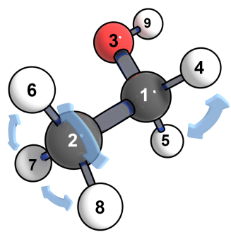
permInvNuclei=4-5.6-7-8
molDescrType=permuted
The permInvNuclei here specifies the atoms to be selected for permutations.
Here the value 4-5.6-7-8 means the hydrogen atoms of the methylene group (CH3CH2OH, the 4th and 5th atoms in the xyz.dat file) can be exchanged, also the hydrogen atoms in the methyl group can be exchanged (CH3CH2OH, the 6th, 7th, and 8th atoms).
The permutational invariant feature provides better accuracy but it’s more computationally costly.
For other molecules, the workflows are the same.
Leave a Reply