MLQD
MLatom can also perform quantum dissipative dynamics with ML via interfaces to the MLQD program.

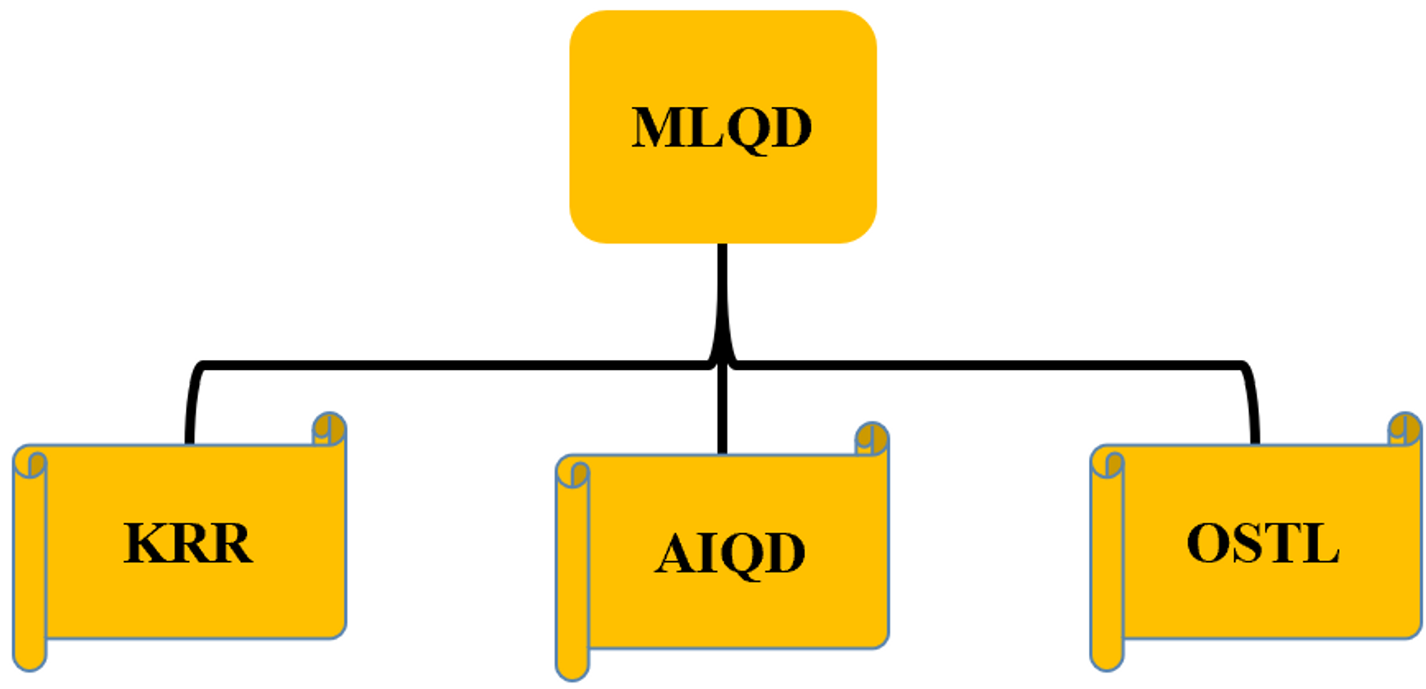
MLQD provides three Machine Learning (ML) methods for propagating quantum dissipative dynamics.
In MLQD, we provide three Machine Learning (ML) methods for propagation Qauntum Dissipative Dynamics
- Kernel Ridge Regression (KRR)-based recursive (iterative) Quantum Dissipative Dynamics method: Here is the corresponding article $\boldsymbol{\rightarrow}$ Speeding up quantum dissipative dynamics of open systems with kernel methods. Recently, we have performed a comparative study where KKR method outperforms NN models, here is the article $\boldsymbol{\rightarrow}$ A comparative study of different machine learning methods for dissipative quantum dynamics
- AIQD non-recursive (non-iterative) approach: Here is the corresponding article Predicting the future of excitation energy transfer in light-harvesting complex with artificial intelligence-based quantum dynamics
- The blazingly fast OSTL non-recursive (non-iterative) approach: Here is the corresponding article One-Shot Trajectory Learning of Open Quantum Systems Dynamics
MLQD provides
- Propagation of dynamics with the existing trained models
- Training convolutional neural networks (CNN) and KRR models on the data
- Transformation of data into input files X and Y
- Optimization of the hyperparameters in CNN and KRR models
Installation and dependencies
Create a conda environment
conda create --name mlqd
Activate the environment
conda activate mlqd
Install the following required dependencies
- tensorflow
conda install -c conda-forge tensorflow - scikit-learn
conda install -c anaconda scikit-learn - hyperopt
conda install -c conda-forge hyperopt - mlatom
pip install mlatom
KRR
Spin-boson model
We will demonstrate the use of KRR model on a two-level spin-boson model.
We consider spin-boson model as was consider in our published study https://iopscience.iop.org/article/10.1088/1367-2630/ac3261
𝐇 = 1/2𝜖𝝈𝑧 + 1/2Δ𝝈𝑥 + ∑𝑘𝜔𝑘𝐛†𝑘𝐛𝑘 + 1/2𝝈𝑧𝐅,
here 𝝈𝑧 and 𝝈𝑥 are the Pauli matrices, i.e., 𝝈𝑧=|𝑒⟩⟨𝑒|−|𝑔⟩⟨𝑔|, 𝝈𝑥=|𝑒⟩⟨𝑔|+|𝑔⟩⟨𝑒|. 𝜖 and Δ are the energy bias and tunneling matrix element, respectively. 𝜔𝑘 is the frequency corresponds to 𝑘 bath mode and 𝐛†𝑘 is the corresponding bath creation operator. 𝐅 is the interaction operator and can be expressed as 𝐅 = ∑𝑘𝑐𝑘2𝜔𝑘√(𝐛𝑘+𝐛†𝑘), where 𝑐𝑘 denotes the coupling strength between system and 𝑘 bath mode. Initially, we consider that the system is in the excited state |𝑒⟩ (by absorbing a photon of energy equal to the energy gap between the two states) and we let the system to be relaxed by exchanging its energy with the bath.
Recursive dynamics
In recursive dynamics, the future dynamics depends in the past dynamics ρ(tn) = f (tn-1). In some traditional quantum dynamics methods such as stochastic equation of motion (SEOM) approach, the noise in long-time dynamics deteriorates the accuracy and a good convergence needs propagation of a large number of trajectories.

What we can do is to train a kernel ridge regression (KRR) model where if we provide a short time dynamics, the model should be able to predict the dynamics beyond it. We demonstarte this on the two-state spin-boson (SB) model. We consider the Drude–Lorentz spectral density
𝐽b(𝜔)=2𝜆𝜔𝛾/(𝜔2+𝛾2),
with 𝛾 as characteristic frequency and 𝜆 as the reorganization energy.

Data generation
We use the Hierarchical equations of motion (HEOM) approach and generate data for all the possible combinations of the following parameters: 𝜖={0,1}, the reorganization energy 𝜆∈{0.1, 0.20.2, 0.30.3, 0.40.4, 0.50.5, 0.60.6, 0.70.7, 0.80.8, 0.90.9, 1.0}, the characteristic frequency 𝛾∈{1, 22, 33, 44, 55, 66, 77, 88, 99, 10}, inverse temperature 𝛽=1/𝑇∈{0.1, 0.250.25, 0.50.5, 0.750.75, 1}. It should be noted that all parameters are in atomic units (a.u.).
We generate 500 trajectories for each case (symmetric and asymmetric) and then train a KRR model on 400 trajectories (keeping 100 trajectories as a test set) for each case. You can grab the trajectories from our QD3SET-1 database, however, here for the sake of demonstration, we provide 20 trajectories. We are also providing the ready made models trained on 400 trajectories for each case. [Coming Soon]
Preparation of the training data
Each trajectory is propagated for t = 20 (a.u.) with the time-step 0.05. For training, you can also use a larger time-step t = 0.1 to minize the cost of training. We take the intial dynamics of time-length tm from each trajectory and then use it an input to predict the dynamics at the next time-step tm+1. We include the dynamics at tm+1 in the input short-time trajectory (dropping the value at t0 to keep the length of the input the same) and then predict the dynamics at tm+2. This process last tills the last time-step.

(Copyright: IOP Publishing https://iopscience.iop.org/article/10.1088/1367-2630/ac3261)
Training a KRR model
Kernel ridge regression (KRR) model approximates a function f(u) which is defined as

where α = {αi} is a vector of regression coefficients αi. We use the Gaussian kernel here To train a KRR model, we use MLatom package (http://mlatom.com/) in the backend.

For the sake of demonstration, we will use the few trajectories provided. Here we take short trajectory of time-length tm = 4.0 (a.u.) as an input-length. In MLatom, we pass it as xlength = 81.
1. With preparation of training data and optimization of the KRR model. MLQD is using MLatom package in the backend
We need to provide the following input to MLatom
MLQD
QDmodel=createQDmodel
QDmodelType=KRR
prepInput=True
dataCol=1
dtype=real
xlength=81
hyperParam=True
systemType=SB
QDmodelOut=KRR_SB_model
Here we are ask MLQD to optimize the hyper parameters hyperParam = True , prepare the input files X and Y from the data prepInput = True , grab the first column of the data files dataCol , grab the real part or imaginary part dtypeand we are also defining the length of the input short trajectories with xlength. We also pass system type as systemType=SB where SB represeny spin-boson model. QDmodelType=KRR pass the type of method which is KRR here. With QDmodel=createQDmodel we ask MLQD to train or create a QD model. The data that we are provided for demonstartion has five columns ( column 0 is time, and column 1 to 4 are population of state-1 ρ11, the off-diagonal term ρ12 , the off-diagonal term ρ21 and population of state-2 ρ22. MLQD will grab the first column and transform into X and Y files and then call MLatom to train a KRR model on the data. However you can pass your own data, just need to mention data path using dataPath=/../../. The trained model will be saved as KRR_SB_model with extension *unf. Please note that MLQD uses MLatom in the backend which will terminate if a saved KRR model is already exist with the same name, so please delete or rename the model before the second run or don’t provide QDmodelOut, MLQD will choose a random name.
2. With preparation of training data but No optimization of the KRR model.
Just need pass False to the hyperParam, i.e., hyperParam = False
MLQD
QDmodel=createQDmodel
QDmodelType=KRR
prepInput=True
dataCol=1
dtype=real
xlength=81
hyperParam=False
systemType=SB
QDmodelOut=KRR_SB_model
3. No preparation of training data and also No optimization of the KRR model.
Just need pass False to the hyperParam and prepInput i.e., hyperParam = False, prepInput = False
MLQD
QDmodel=createQDmodel
QDmodelType=KRR
prepInput=False
XfileIn=x_data
YfileIn=y_data
hyperParam=False
systemType=SB
QDmodelOut=KRR_SB_model
With XfileIn and YfileIn we pass the X and Y files.
Propagating dynamics with the trained KRR model
Let’s propagate dynamics with the above trained KRR model trained on site-1 population. We provide a test file using XfileIn which has an unseen short time trajectory (of the same time-length as was adopted during the training). We feed this short-time dynamics to the trained KRR model and we hope that it will predict the long dynamics. The short-time trajectoy is passed as a txt file.
MLQD
time=20
time_step=0.05
QDmodel=useQDmodel
QDmodelType=KRR
XfileIn=test_set/sb/state_1_pop.txt
systemType=SB
QDmodelIn=KRR_SB_model
QDtrajOut=KRR_trajectory
where time is the propagation time which is in atomic units (a.u.) for spin-boson model. time_step pass the time step for propagation which should be equal to training data time-step. With QDmodel=useQDmodel we are asking MLQD to use a provided trained model. QDmodelType=KRR pass the type of method which is KRR here. XfileIn=test_set/sb/state_1_pop.txt pass the file with short time trajectory equal to the time-length tm = 81. We passs the trained KRR model with QDmodelIn=KRR_SB_model (with no extension). The predicted dynamics will be saved as QDtrajOut=KRR_trajectory which is optional, if you don’t pass it, the MLQD will generate a random name. After successful prediction of dynamics, you can plot it against the reference trajectory.
2_epsilon-0.0_Delta-1.0_lambda-0.1_gamma-4.0_beta-1.0.npy

OSTL Approach
In One-shot Trajectory Learning (OSTL) approach, we prepare our training data using parameters {𝜖, Δ, 𝛾, 𝜆, 𝛽}

where N is the dimension of the reduced density matrix and calligraphic R and calligraphic I represent the real and imaginary parts of the off-diagonal terms, respectively.
More details are here
One-Shot Trajectory Learning of Open Quantum Systems Dynamics
1. Training with preparation of training data and optimization of the CNN model
For the sake of demonstration, we provid 20 trajectories from our QD3SET-1 database which will be extracted by default. Each trajectory is propagated with HEOM method upto t= 20 (a.u.) with time-step dt = 0.05. However, you can also pass your own data using dataPath=../../..
MLQD
n_states=2
QDmodel=createQDmodel
QDmodelType=OSTL
prepInput=True
energyNorm=1.0
DeltaNorm=1.0
gammaNorm=10
lambNorm=1.0
tempNorm=1.0
systemType=SB
hyperParam=True
patience=10
QDmodelOut=OSTL_SB_model
n_states pass the number of states for SB or number of sites in case of FMO. Default is 2 (SB) and 7 (FMO). In OSTL approach, we normalize teh values between 0 and 1. energyNorm is normalizer for energy difference 𝜖. DeltaNorm is normalizer for Δ. Default value is 1.0. gammaNorm is normalizer for Characteristic frequency 𝛾. Default value is 10 in the case of spin-boson model. lambNorm is normalizer for System-bath coupling strength 𝜆. Default value is 1. tempNorm is normalizer for inverse temperature 𝛽 . Default value is 1. patience is the patience for early stopping in CNN training. Here we are ask MLQD to optimize the hyper parameters hyperParam = True , prepare the input files X and Y from the data prepInput = True . We also pass system type as systemType=SB where SB represeny spin-boson model. QDmodelType=OSTL pass the type of method which is OSTL here. With QDmodel=createQDmodel we ask MLQD to train or create a QD model. MLQD will save the model as OSTL_SB_model, you may not provide QDmodelOut, MLQD will choose a random name.
2. Training with preparation of training data but no optimization of the CNN model
pass hyperParam=False
MLQD
n_states=2
QDmodel=createQDmodel
QDmodelType=OSTL
prepInput=True
energyNorm=1.0
DeltaNorm=1.0
gammaNorm=10
lambNorm=1.0
tempNorm=1.0
systemType=SB
hyperParam=False
patience=10
QDmodelOut=OSTL_SB_model
3. Training with no preparation of training data and no optimization of the CNN model
pass prepInput=False and also need to pass the X and Y files using XfileIn and YfileIn
MLQD
n_states=2
QDmodel=createQDmodel
QDmodelType=OSTL
prepInput=True
XfileIn=x_data
YfileIn=y_data
systemType=SB
hyperParam=False
patience=10
QDmodelOut=OSTL_SB_model
Propagating dynamics with the trained OSTL model
Here we will demonstrate how to propagate dynamics with the model we trained in above steps. We will provide the simulation parameters and the OSTL will predict the corresponding dynamics
MLQD
n_states=2
time=20
time_step=0.05
energyDiff=1.0
Delta=1.0
gamma=4.0
lamb=0.1
temp=1.0
QDmodel=useQDmodel
QDmodelType=OSTL
energyNorm=1.0
DeltaNorm=1.0
gammaNorm=10
lambNorm=1.0
tempNorm=1.0
systemType=SB
QDmodelIn=OSTL_SB_model.hdf5
QDtrajOut=Qd_trajectory
Here we pass the values of 𝜖, Δ, 𝛾, 𝜆, and 𝛽. Propagation time is 20 which should be equal to the training time and also the time_step should be equal to the time-step used in the training data. The predicted dynamics will be saved as QDtrajOut=KRR_trajectory which is optional, if you don’t pass it, the MLQD will generate a random name. Now you can plot the dynamics against the test trajectory 2_epsilon-0.0_Delta-1.0_lambda-0.1_gamma-4.0_beta-1.0.npy
AIQD
We prepare our training using parameters 𝜖, Δ, 𝛾, 𝜆, T and f(t) where f(t) is the logistic function to normalize the dimension of time, i.e.,
f(t) = a/(1 + b exp(-(t + c)/d))
where a, b, c and d are constants. Check out the Supplementary Figure 3 of our AIQD papar Predicting the future of excitation energy transfer in light-harvesting complex with artificial intelligence-based quantum dynamics.
For each time-step, the AIQD approach predicts and was trained on the corresponding reduced density matrix in the following format

where N is the dimension of the reduced density matrix and calligraphic R and calligraphic I represent the real and imaginary parts of the off-diagonal terms, respectively.
1. Training with preparation of training data and optimization of the CNN model
MLQD
n_states=2
time=20
time_step=0.05
QDmodel=createQDmodel
QDmodelType=AIQD
prepInput=True
numLogf=10
LogCa=1.0
LogCb=15.0
LogCc=-1.0
LogCd=1.0
energyNorm=1.0
DeltaNorm=1.0
gammaNorm=10
lambNorm=1.0
tempNorm=1.0
systemType=SB
hyperParam=True
patience=10
QDmodelOut=AIQD_SB_model
Here we are ask MLQD to optimize the hyper parameters hyperParam = True , prepare the input files X and Y from the data prepInput = True . We also pass system type as systemType=SB where SB represeny spin-boson model. QDmodelType=AIQD pass the type of method which is AIQD here.
n_states pass the number of states for SB or number of sites in case of FMO. Default is 2 (SB) and 7 (FMO). In OSTL approach, we normalize the values between 0 and 1. energyNorm is a normalizer for energy difference 𝜖. DeltaNorm is normalizer for Δ. Default value is 1.0. gammaNorm is normalizer for Characteristic frequency 𝛾, which by default is equal to 10 in the case of spin-boson model. lambNorm is normalizer for System-bath coupling strength 𝜆. Default value is 1. tempNorm is normalizer for inverse temperature 𝛽. Default value is 1. patience is the patience for early stopping in CNN training.
numLogf Number of Logistic function for the normalization of time dimension. Default value is 1.0. LogCa, LogCb, LogCc and LogCd pass the values for a, b, c, and d are constants. Here time pass the time-length of the trajectory so it can be normalized accordingly and the time-step pass the time-step. QDmodelOut=AIQD_SB_model(which is optional) is providing a name to save the model at.
2. Training with preparation of training data but no optimization of the CNN model
pass hyperParam=False
MLQD
n_states=2
time=20
time_step=0.05
QDmodel=createQDmodel
QDmodelType=AIQD
prepInput=True
numLogf=10
LogCa=1.0
LogCb=15.0
LogCc=-1.0
LogCd=1.0
energyNorm=1.0
DeltaNorm=1.0
gammaNorm=10
lambNorm=1.0
tempNorm=1.0
systemType=SB
hyperParam=False
patience=10
QDmodelOut=AIQD_SB_model
3. Training with no preparation of training data and no optimization of the CNN model
pass prepInput=False and also need to pass the X and Y files using XfileIn and YfileIn
MLQD
n_states=2
time=20
time_step=0.05
QDmodel=createQDmodel
QDmodelType=AIQD
prepInput=False
XfileIn=x_data
YfileIn=y_data
hyperParam=False
patience=10
QDmodelOut=AIQD_SB_model
Propagating dynamics with the trained AIQD model
Here we will demonstrate how to propagate dynamics with the model we trained in above steps. We will provide the simulation parameters and the OSTL will predict the corresponding dynamics
MLQD
n_states=2
time=20
time_step=0.05
energyDiff=1.0
Delta=1.0
gamma=4.0
lamb=0.1
temp=1.0
QDmodel=useQDmodel
QDmodelType=OSTL
energyNorm=1.0
DeltaNorm=1.0
gammaNorm=10
lambNorm=1.0
tempNorm=1.0
numLogf=10
LogCa=1.0
LogCb=15.0
LogCc=-1.0
LogCd=1.0
systemType=SB
QDmodelIn=AIQD_SB_model.hdf5
QDtrajOut=Qd_trajectory
The predicted dynamics will be saved as QDtrajOut=KRR_trajectory which is optional, if you don’t pass it, the MLQD will generate a random name. Now you can plot it against the reference trajectory 2_epsilon-0.0_Delta-1.0_lambda-0.1_gamma-4.0_beta-1.0.npy